

An audio meter becomes useful when it stops pretending that every signal question has one answer.
It is tempting to ask whether a recording is "loud," then look for a single number that settles it. But loudness, headroom, spectral balance, transient behavior, and waveform shape are different properties. A mix can be loud but leave generous peak margin. A vocal can show a clean spectrum while carrying an unstable DC offset. A short drum hit can look harmless in an averaged level reading and still challenge an encoder.
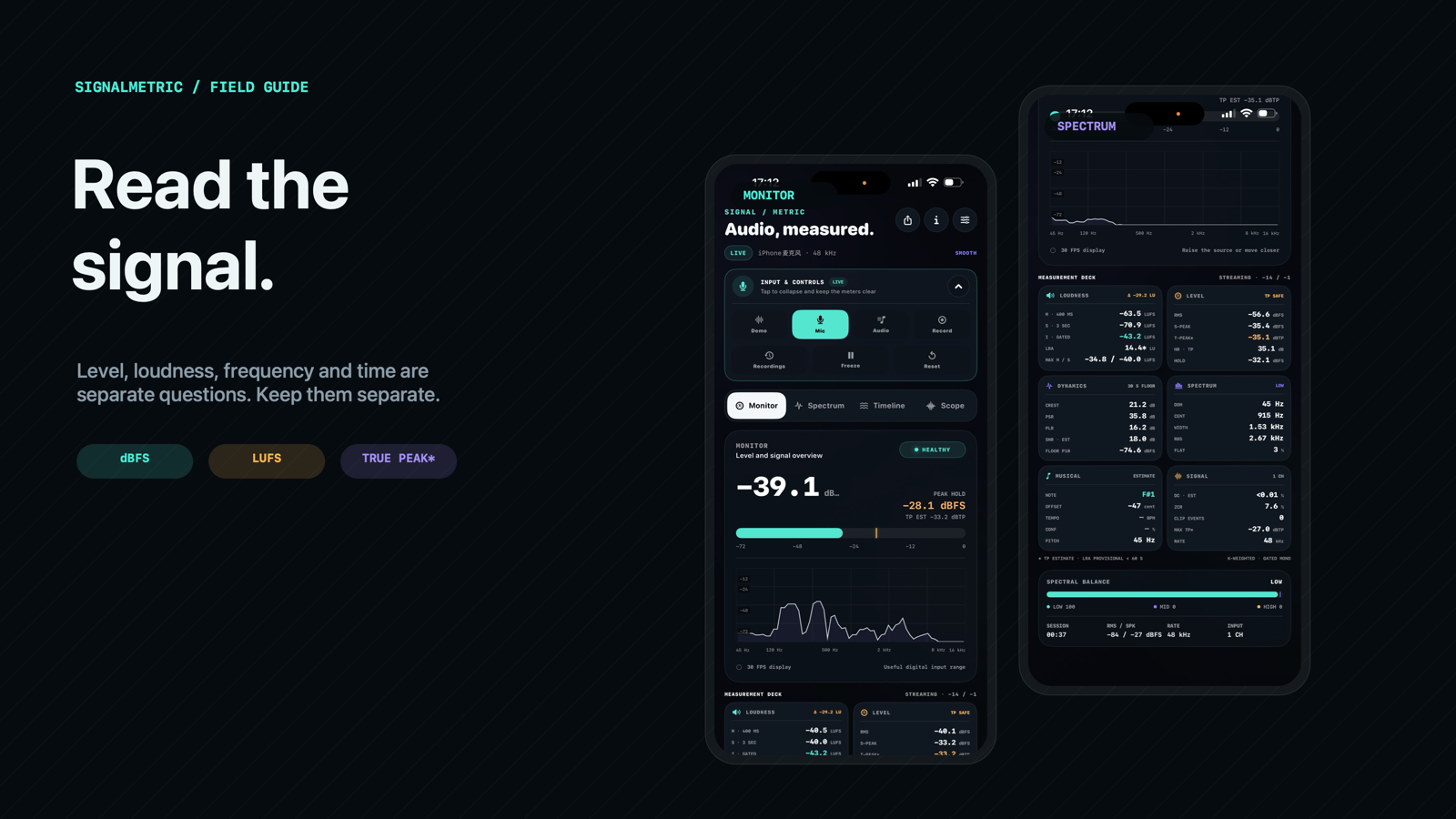
SignalMetric is built around that separation. The Monitor, Spectrum, Timeline, and Scope are four ways to interrogate the same source. Each is deliberately narrow enough to answer one question well.
Swipe horizontally to explore the diagram
This diagram could not be rendered. Its source is still available below.
View diagram source
flowchart TD
    A[Audio source] --> B[Level and peaks]
    A --> C[Perceived loudness]
    A --> D[Frequency content]
    A --> E[Time-domain shape]
    B --> B1[dBFS, Sample Peak, True Peak estimate, Headroom]
    C --> C1[Momentary, Short-Term, Integrated LUFS, LRA]
    D --> D1[FFT trace, components, centroid, spectral history]
    E --> E1[Triggered waveform, DC offset, zero-crossing rate]
The guide below is not a list to memorize. It is a way to choose the next view when a number makes you curious.
Start with the digital ceiling
dBFS means decibels relative to full scale. In a digital signal, 0 dBFS is the ceiling. A reading such as -18 dBFS describes the signal's level below that maximum representable sample value; it does not describe the acoustic sound pressure in a room.
That distinction matters. A phone microphone, a USB interface, and an imported file can all produce a dBFS reading, but they do not become calibrated sound-pressure meters merely because the number is displayed in decibels. SignalMetric keeps its live readings in the digital domain and does not add a pretend SPL offset.
Two level values are particularly useful:
Swipe horizontally to see all columns
| Reading | What it asks | When to look at it |
|---|---|---|
| RMS dBFS | How much average signal energy is present in this analysis window? | Setting a usable input level or comparing sustained sections. |
| Sample Peak dBFS | How close did an observed sample get to digital full scale? | Checking immediate headroom and obvious clipping risk. |
RMS is not a replacement for peak. A sparse percussion part may have a moderate RMS value while its transients arrive much closer to the ceiling. Conversely, a heavily compressed source may keep RMS and peak much closer together. SignalMetric also shows crest factor, the gap between instantaneous peak and RMS, because that gap is often more revealing than either number alone.
Sample Peak and True Peak answer neighboring questions
Sample Peak inspects the sample points that were delivered to the analyzer. Between those points, a reconstructed waveform can rise higher. This is why an export that never visibly reaches 0 dBFS may still cause trouble later in a conversion or playback chain.
SignalMetric reports a 4x inter-sample True Peak estimate in dBTP. The word estimate is important. The app performs windowed-sinc reconstruction between samples to provide useful evidence about likely inter-sample overs, but it does not claim a certified delivery-QC result.
Use the pair like this:
- Look at Sample Peak to see the observed sample ceiling.
- Look at True Peak estimate to see whether reconstruction may reduce the remaining margin.
- Look at headroom to turn that margin into a direct operational question: how much room remains before the chosen ceiling?
- If either number is unexpectedly hot, move to Scope or Spectrum to find out whether the source is a transient, a narrow resonance, or a sustained balance problem.
For a general streaming reference, SignalMetric can display -14 LUFS / -1 dBTP; its EBU R128 and ATSC A/85 profiles are presentation references, not transformations applied to the audio. The source remains untouched.
LUFS is about duration, not a faster peak meter
Loudness has a different job from peak measurement. It estimates how programme level accumulates over time after K-weighting, which is why it needs time windows and gating rather than a single instantaneous amplitude.
SignalMetric exposes four related readings:
- Momentary LUFS uses a 400 ms window. It is useful for following a phrase or a brief edit.
- Short-Term LUFS uses a 3 s window. It is often easier to read for a chorus, a spoken sentence, or a sustained ambience.
- Integrated LUFS aggregates a session through absolute and relative gates. It should settle over meaningful programme duration, not be treated as a verdict on the first second of audio.
- Loudness Range (LRA) describes the spread of gated Short-Term loudness. SignalMetric marks it as provisional before 60 seconds because a short listen cannot establish a meaningful range.
The implementation follows the timing and gating vocabulary of ITU-R BS.1770 for its explicit mono analysis signal. That phrasing is precise: multi-channel files are folded to mono for analysis, and the app does not represent itself as a certified compliance tool.
The most practical habit is to compare loudness with peak margin, not in isolation. A Short-Term reading near a target can coexist with a True Peak estimate that leaves too little margin. That is where PSR and PLR help: both express a relationship between loudness and peak behavior, but they refer to different time scopes.
The spectrum says where the energy lives
When a signal feels dull, brittle, boxy, or unstable, a level meter cannot tell you why. That is a frequency question.
SignalMetric analyzes a 2,048-sample mono window with a Hanning window and displays a logarithmic 64-band trace across the usable analysis range. The log axis matters because musical and speech perception care about relative frequency spacing: the room between 100 Hz and 200 Hz deserves more visual attention than the same linear distance between 10,100 Hz and 10,200 Hz.
The Spectrum view has two layers:
- The trace shows the broader energy distribution in dBFS.
- The component view selects up to six strong local FFT peaks and reports interpolated frequency, level, period, nearest note, and a conditional harmonic fit.
Those components are an explanation of prominent peaks, not a claim that the app has reconstructed the entire signal into six perfect sine waves. Peak selection suppresses nearby window artifacts, and the presentation is smoothed so a tiny change in rank does not make the grid flicker every frame.
Three spectrum statistics make quick comparison easier:
Swipe horizontally to see all columns
| Statistic | A useful reading of it |
|---|---|
| Centroid | A high centroid means more energy is concentrated toward higher frequencies. It is a clue, not a brightness score. |
| Bandwidth | A wider spread suggests energy occupies more of the available spectrum. |
| 85% roll-off | The frequency below which most spectral energy sits. Useful for comparing sources with similar overall level. |
If you want to understand a source more deeply, drag across the Spectrum view. The selected frequency becomes the shared inspection point rather than a loose cursor with no relationship to the component readout.
Timeline and Scope restore the missing dimension
A static spectrum is a snapshot. It can hide whether a resonance appears only on certain words, whether a low-frequency hit drifts into the mix, or whether the source changed after an edit.
The Timeline retains a bounded 30-second spectral history at eight published frames per second, for at most 240 columns. It is intentionally a recent-history instrument, not a recording archive. Use it when the question is "when did that band appear?" rather than "what is happening right now?"
The Scope answers a different question again. It draws a triggered, 256-bin time-domain envelope. This is useful when you need to see attack shape, periodicity, asymmetry, or a discontinuity that is difficult to understand from frequency data alone. DC offset and zero-crossing rate sit beside it because they describe signal behavior at the sample level:
- DC offset shows whether the waveform is centered around zero.
- Zero-crossing rate shows how often the signal changes sign. It can be a helpful texture clue, but it is not a genre label or a substitute for spectral analysis.
- Clipping events count samples that reach the digital ceiling, keeping a session-level record of a problem that may be too brief to catch by eye.
A simple inspection order
There is no universal meter-reading ritual, but this order works well for a live mic, an imported clip, or a local recording:
- Start in Monitor. Confirm there is a usable signal, note RMS, Sample Peak, True Peak estimate, and headroom.
- Check Short-Term LUFS and the peak relationship if the goal involves programme level rather than input setup.
- Open Spectrum when the balance needs an explanation. Inspect a suspicious band instead of guessing from the overall trace.
- Open Timeline if the issue changes over time.
- Open Scope if the signal itself looks suspect: an abrupt transient, offset waveform, unstable trigger, or clipping event.
The same workflow applies whether the source is a permission-free demo, a microphone, or a local file. The SignalMetric product guide has the full feature overview, but the core idea is simpler: let the question choose the instrument.
What the meter should not promise
A meter earns trust by showing its boundary as clearly as its result.
SignalMetric reports dBFS and BS.1770-aligned mono loudness values. Its True Peak value remains visibly marked as an estimate. Tempo and pitch are withheld or marked approximate when confidence is weak. The built-in microphone is not presented as calibrated SPL hardware, and no displayed number is a substitute for validated equipment in legal, occupational, or hearing-safety work.
That restraint is not a missing feature. It keeps a useful observation from becoming a misleading conclusion.